
Comprehensive Biostatistics and Computer Notes – Units 1 to 4
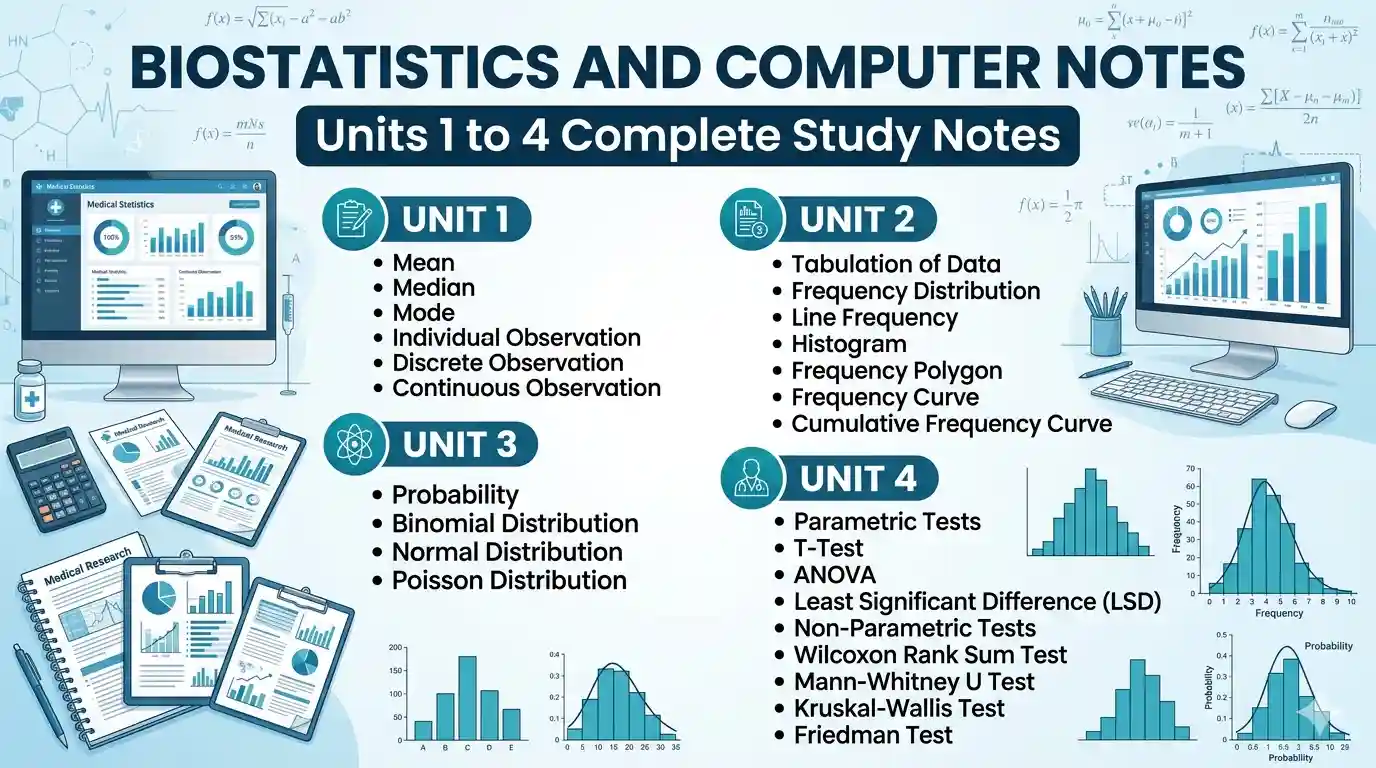
Detailed Notes Pdf – BIOSTATISTICS AND COMPUTER APPLICATIONS
Short Notes -✅ UNIT 1
1. Definition & Calculation of Mean (Direct Method, Shortcut Method and Step Deviation Method)➛
The mean, also known as the arithmetic mean or average, is a measure of the central tendency of a dataset or a population. It represents the sum of all values divided by the number of values.
In simpler terms, the mean is a way to describe the “typical” value in a dataset. It’s a single value that represents the entire dataset, and it’s often used to understand the general trend or pattern in the data.
The mean is sensitive to extreme values (outliers) in the data, and it’s not always the best representation of the data, especially when the data is skewed or has outliers. In such cases, other measures like the median or mode might be more appropriate.
Formula
Mean = (Σx) / n
Where:
- Σx = Sum of all values
- n = Number of values
Example
Numbers: 2, 4, 6, 8, 10
Mean = (2 + 4 + 6 + 8 + 10) / 5
Mean = 30 / 5 = 6
Direct Method
The direct method involves adding up all the values in a dataset and dividing by the number of values.
Formula
Mean = (Σx) / n
Where:
- Σx = Sum of all values
- n = Number of values
Example
Find the mean of 2, 4, 6, 8, 10
Σx = 2 + 4 + 6 + 8 + 10 = 30
n = 5
Mean = 30 / 5 = 6
Shortcut Method
The shortcut method involves finding the mean of a dataset by first finding the mean of a smaller subset of the data and then adjusting for the remaining values.
Formula
Mean = (Σx + (n – m) × A) / n
Where:
- Σx = Sum of a smaller subset of values
- n = Total number of values
- m = Number of values in the subset
- A = Mean of the subset
Example
Find the mean of 2, 4, 6, 8, 10 using subset 2, 4, 6
Σx = 12
n = 5
m = 3
A = 12 / 3 = 4
Mean = (12 + (5 – 3) × 4) / 5
= (12 + 8) / 5
= 20 / 5
= 4
Step Deviation Method
The step deviation method involves finding the mean by first finding the deviation of each value from an assumed mean, then finding the mean of these deviations, and finally adjusting the assumed mean.
Formula
Mean = A + (Σd / n)
Where:
- A = Assumed mean
- Σd = Sum of deviations from A
- n = Number of values
Example
Assumed Mean = 5
Deviations:
- (2 – 5) = -3
- (4 – 5) = -1
- (6 – 5) = 1
- (8 – 5) = 3
- (10 – 5) = 5
Σd = 5
Mean = 5 + (5 / 5)
Mean = 6
2. Mode and Median
In biostatistics, the median is the middlemost value in the ordered list of observations, and the mode is the most frequently occurring value.
Mode
The mode is the most frequently occurring value in a dataset.
Steps to Calculate Mode
- Arrange the data in ascending or descending order.
- Count the frequency of each value.
- Identify the value with the highest frequency.
- The value with the highest frequency is the mode.
Example
Data: 1, 2, 3, 4, 4, 4, 5, 6
Mode = 4
Bimodal Distribution Example
Data: 1, 2, 2, 3, 3, 3, 4, 4, 4
Modes = 3 and 4
Median
The median is the middle value when the dataset is arranged in ascending or descending order.
Steps to Calculate Median
- Arrange data in ascending order.
- Count the number of observations (n).
- If n is odd, median is the middle value.
- If n is even, median is the average of the two middle values.
Example (Odd)
Data: 1, 3, 5, 7, 9
Median = 5
Example (Even)
Data: 1, 3, 5, 7, 9, 11
Median = (5 + 7) / 2
Median = 6
3. Individual Observation
An individual observation is a single data point or measurement collected from a single subject, participant, or unit of analysis in a study or experiment.
Examples include:
- Participant ID
- Age
- Gender
- Weight
- Survey responses
Individual observations are the building blocks of statistical analysis and are used to calculate summary statistics, perform hypothesis testing, and model relationships between variables.
4. Discrete Observation
A discrete observation is a type of individual observation that can only take on specific, distinct, and countable values.
Examples:
- Gender
- Color
- Number of children
- Yes/No responses
- Income categories
Discrete observations are commonly analyzed using:
- Frequency counts
- Percentages
- Chi-square tests
5. Continuous Observation
A continuous observation can take any value within a certain range or interval.
Examples:
- Height
- Weight
- Blood Pressure
- Temperature
- Time
- Distance
Characteristics:
- Can take any value within a range
- Measured on a continuous scale
- Can include decimal values
- Analyzed using mean, standard deviation and regression analysis
✅ UNIT 2
1. Tabulation of Data and Graphical Presentation of Frequency Distribution
Tabulation of Data
Tabulation involves organizing and summarizing data into tables.
Common Tables:
- Frequency Tables
- Contingency Tables
- Descriptive Statistics Tables
Graphical Presentation of Frequency Distribution
Common Graphs:
- Histogram
- Bar Chart
- Pie Chart
- Box Plot
Advantages:
- Helps identify trends and patterns
- Easy interpretation of data
- Supports decision-making
2. Line Frequency
Line frequency (Frequency Polygon) is a graphical representation of frequency distribution using connected lines.
Characteristics:
- X-axis represents values or ranges.
- Y-axis represents frequencies.
- Points are connected by straight lines.
Uses:
- Displaying distribution shape
- Identifying modes and outliers
- Comparing groups
3. Histogram (Equal and Unequal Class Intervals)
A histogram is a graphical representation of a frequency distribution using bars.
Equal Class Intervals
All class intervals have the same width.
Example:
| Class Interval | Frequency |
|---|---|
| 0–10 | 5 |
| 11–20 | 8 |
| 21–30 | 12 |
| 31–40 | 10 |
| 41–50 | 7 |
Unequal Class Intervals
Class intervals have different widths.
Example:
| Class Interval | Frequency |
|---|---|
| 0–5 | 3 |
| 6–15 | 8 |
| 16–30 | 15 |
| 31–50 | 12 |
| 51–100 | 5 |
4. Inclusive Data and Mid Value
Inclusive Data
Inclusive data includes all values without gaps or overlaps.
Example:
0–5, 5–10
Mid Value
The midpoint of a class interval.
Formula:
Mid Value = (Upper Limit + Lower Limit) / 2
Example:
Class Interval 0–5
Mid Value = 2.5
5. Frequency Polygon
A frequency polygon is constructed by:
- Plotting class mid-values on the x-axis.
- Plotting frequencies on the y-axis.
- Connecting points with straight lines.
Uses:
- Visualizing distribution
- Comparing variables
- Identifying patterns
6. Frequency Curve
A frequency curve is a smooth graphical representation of a frequency distribution.
Uses:
- Identifying skewness
- Detecting peaks and troughs
- Understanding spread of data
7. Cumulative Frequency Curve (Ogive)
A cumulative frequency curve shows cumulative frequencies against upper class limits.
Applications:
- Finding median
- Determining percentiles
- Identifying distribution characteristics
✅ UNIT 3
1. Probability
Probability is a measure of the likelihood of an event occurring.
Range:
- 0 = Impossible Event
- 1 = Certain Event
Formula:
P(A) = Number of Favorable Outcomes / Total Number of Possible Outcomes
Applications:
- Statistics
- Engineering
- Finance
- Insurance
- Medicine
2. Definition of Probability
Probability is a number between 0 and 1 representing the chance of occurrence of an event.
Formula:
P(A) = Favorable Outcomes / Total Outcomes
Properties of Probability
- Non-Negativity
- Normalization
- Countable Additivity
- Monotonicity
- Subadditivity
- Conditional Probability
- Independence
- Multiplication Rule
- Law of Total Probability
- Bayes’ Theorem
3. Binomial Distribution
The binomial distribution models the number of successes in a fixed number of independent trials.
Parameters:
- n = Number of trials
- p = Probability of success
Properties
- Mean = np
- Variance = np(1-p)
- Standard Deviation = √np(1-p)
Applications:
- Coin Tossing
- Quality Control
- Medical Research
4. Normal Distribution
The normal distribution (Gaussian Distribution) is a symmetrical bell-shaped probability distribution.
Characteristics
- Mean = Median = Mode
- Symmetrical around mean
- Continuous distribution
Important Percentages
- 68% within 1 SD
- 95% within 2 SD
- 99.7% within 3 SD
Applications:
- Human height
- IQ scores
- Measurement errors
- Medical statistics
5. Poisson Distribution
The Poisson distribution models the number of events occurring within a fixed interval.
Parameter:
λ (Lambda)
Formula
P(X = k) = (e^-λ × λ^k) / k!
Properties
- Mean = λ
- Variance = λ
- Mode = λ
Applications:
- Disease occurrence
- Customer arrivals
- Manufacturing defects
6. Properties and Problems of Poisson Distribution
Properties:
- Mean = λ
- Variance = λ
- Memoryless nature
- Summation property
- Limiting case of Binomial Distribution
- Approximation to rare event probability
Practice Problems:
- Manufacturing defects problem
- Call center arrival problem
- Disease occurrence problem
- Quality control problem
- Banking customer arrival problem
✅UNIT 4
1. Parametric Tests
Parametric tests assume a specific distribution of data.
Examples:
- T-Test
- ANOVA
- Regression Analysis
- Chi-Square Test
- F-Test
Assumptions
- Normality
- Equal Variances
- Independence
2. T-Test (One Sample, Unpaired/Pooled and Paired)
The T-Test determines whether a significant difference exists between means.
Types
One-Sample T-Test
Compares sample mean with population mean.
Unpaired/Pooled T-Test
Compares means of two independent groups.
Paired T-Test
Compares means of two related groups.
Applications:
- Clinical studies
- Educational research
- Experimental analysis
3. ANOVA (One-Way and Two-Way)
ANOVA compares means of multiple groups.
One-Way ANOVA
One independent variable.
Example:
Comparing scores of three classes.
Two-Way ANOVA
Two independent variables.
Example:
Comparing scores by gender and age group.
Assumptions
- Normality
- Equal Variances
- Independence
4. Least Significant Difference (LSD)
LSD is a post-hoc test used after ANOVA to determine which groups differ significantly.
Formula
LSD = t × √(2 × MSE / n)
Where:
- t = Critical value
- MSE = Mean Square Error
- n = Sample size
Non-Parametric Tests
Non-parametric tests do not require normal distribution assumptions.
Examples:
- Wilcoxon Rank-Sum Test
- Mann-Whitney U Test
- Kruskal-Wallis Test
- Friedman Test
- Chi-Square Test
- Sign Test
1. Wilcoxon Rank-Sum Test
Used to compare two independent groups.
Assumptions:
- Independent observations
- Ordinal or continuous data
2. Mann-Whitney U Test
Alternative to Independent Samples T-Test.
Used when normality assumptions are not met.
3. Kruskal-Wallis Test
Used to compare three or more independent groups.
Alternative to One-Way ANOVA.
4. Friedman Test
Used to compare three or more related groups.
Alternative to Repeated Measures ANOVA.
Assumptions:
- Related observations
- Ordinal or continuous data
Operation Theatre Technology Notes : Powered Surgical Instruments and Specialized Surgical Equipment

Nice